Quantum Cascade Laser
Figure of Merit Derivation

1 Figure of merit the easy way

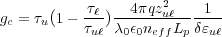
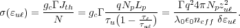
The figure of merit (FoM) for a quantum cascade (QC) laser (QCL) is a tool used to maximize performance from a QC design. The FoM represents the parameters from the QC laser gain coefficient that are affected by the quantum design of a QC structure. The QCL gain coefficient is generally given as:

(1)

where τ_u is the lifetime of the upper laser state, τ_ℓ is the lifetime of the lower laser state, q is the electron charge, τ_uℓ is the transition time between the upper and lower laser state, z_uℓ is the optical dipole matrix element (having units of length), λ₀ is the free space wavelength of the lasing transition, n_eff is the effective refractive index of the optical mode, L_p is the length of a single active-injector region period, and δɛ_uℓ is the full-width-at-half-maximum (FWHM) of transition’s spontaneous emission (usually taken as the measured FWHM of a QC structure’s electroluminescence, and in units of energy). The gain coefficient as defined this way has units of , which is generally .

Since the optical dipole matrix element z_uℓ and the energy state lifetimes τ_i are QC design-dependent parameters, the most direct approach to deriving a FoM is simply to pull these factors from the gain coefficient.

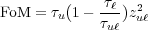(2)

Thus, the FoM has units of time x length²; the standard units are ps Ų. While this is the simplest method for deriving a FoM, it has severe limitations when practically implemented. QC lasers after all, comprise a system of coupled quantum wells with significant intermixing (anticrossing) of quantum states; in Eq. (2), we have assumed only a single upper laser state and a single lower laser state.

2 Intermixed lower energy states

For a proper calculation of the laser gain coefficient—and thus FoM—we must include all optical transitions that might contribute photons into the lasing mode. One might address this problem by perturbing the field at which the FoM parameters are calculated, so as to prevent the upper and lower laser states from intermixing with nearby states. However, the FoM itself is a field-dependent parameter, so this approach is not ideal for calculating laser gain at current turn-on (i.e., the design field).

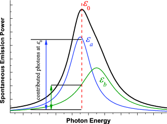
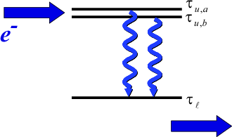
To more broadly address the problem of multiple charge carrier transitions contributing photons to the lasing mode, we need to consider each potential transition’s contribution to the optical gain. As an example, let’s examine an optical transition with one upper energy state and two closely spaced, intermixed lower energy states.

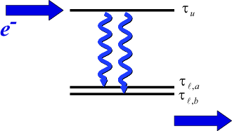
We need to remember that each transition has its own spontaneous emission spectrum with a finite FWHM; in intersubband heterostructure emitters, a good estimate for δɛ_uℓ is 10% of the transition energy. If the two transitions are close enough together, the spontaneous emission will overlap in energy. Let’s assume the spontaneous emission lineshape for a transition with energy ɛ_uℓ has a Lorentzian form.

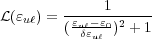(3)

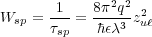
Here, ɛ₀ is the lasing photon energy. Now, each transition will be able to contribute to lasing. The lasing wavelength would not be exactly that of a single optical transition, but somewhere between the two transitions. To find the lasing wavelength, we need to keep in mind that the transitions might have different spontaneous emission rates. That is, one transition might be able to emit photons faster than the other. The spontaneous emission rate W_sp [] is the inverse of the spontaneous emission lifetime τ_sp [time].

(4)

Notice that the rate, or the strength of the transition, is proportional to z_uℓ². If we add up the spontaneous emission spectrum of each transition multiplied by z_uℓ², the peak gain and thus the lasing energy ɛ₀ can be found.

(5)

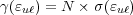
Now that we know what the lasing energy is going to be, let’s look at stimulated emission for each of the transitions. Gain γ [] is simply the charge carrier population difference N = N_u - N_ℓ [] times the transition cross-section σ [area].

(6)

Let’s take each of the two contributions to γ individually. In a simple two level optical transition system with an upper state pumped at rate R_u [], the carrier population difference is

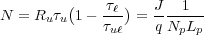(7)

where J is pumping current density [] and N_p is the number of active region-injector periods in the QCL active core. The transition cross-section can be found by recognizing that, at threshold where optical gain clamps,

(8)

where α_total is the total optical loss (waveguide and mirror loss), Γ is the gain region confinement factor for the optical mode in the waveguide, and J_th is the threshold current density []. By applying Eqs. (1), (6) and (7) to Eq. (8), we get

(9)

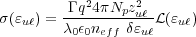
While this is close for the gain cross-section, we’ve got one correction to make. The gain coefficient from Eq. (1) was derived assuming two discreet states. To correct for this, we need to multiply the original g_c by our lineshape function (ɛ_uℓ) from Eq. (3). Thus, we get the quantum cascade laser transition cross-section.

(10)

Now, getting back to our example with one upper energy state and two closely spaced lower energy states, we can pull from the components of Eq. (6) those elements that are influenced by quantum design.

FoM	= τu1 -zuℓ,a2(ɛ uℓ,a) + τu1 -zuℓ,b2(ɛ uℓ,b)
	= ∑ ℓτu1 -zuℓ2(ɛ uℓ)	(11)

3 Intermixed upper energy states

Calculating a proper FoM for energy transitions with upper state intermixing takes consideration similar to the lower state intermixing case. However, with upper state intermixing, we have an additional complication. We cannot assume that each upper energy state is equally populated with electrons; the relative populations of each upper state will influence the total gain contributed by that transition.

Recall that our basic relation for gain,

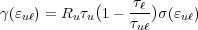(12)

has a term R_u that describes the rate at which the upper energy level u is populated with electrons. For a FoM calculation, where we are focused on obtaining a number that allows us to compare different QC designs, we are not concerned about the absolute pumping rate. Rather, what we need is a weighting factor that reflects the relative population of each of the upper energy states. Now, we can write our FoM as

(13)

with an upper state weighting factor C_u. As we’ve previously shown, the pumping rate R_u of an energy state is proportional to the current density passing through the state. In a QCL system with strong coupling between energy states,

(14)

where n_u is the sheet density [] of electrons populating the state. Thus, our weighting factor C_u ∝ n_u∕τ_u. The energy state population n_u follows the Fermi-Dirac distribution

(15)

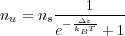
where Δɛ = ɛ_u -ɛ_F is approximately the energy difference between the state u and the injector ground state, k_B is the Boltzmann constant, and T is temperature. For most quantum cascade laser systems, with relatively low doping (carrier densities) and high temperatures, the Fermi distribution is well-approximated by the Boltzmann distribution, so

(16)

and

(17)

Since C_u is a weighting factor, the restriction ∑ _uC_u = 1 must hold.

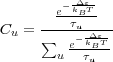(18)

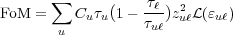
Finally, we arrive at the general equation for FoM by combining Eqs. (11) and (13), the generalized cases for transitions between intermixed upper and lower energy states.

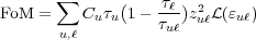(19)